CG(描画)

listplot, pointplot

リスト構造にある離散的なデータはlistplotで表示してくれる．listplotは受け取ったlistの要素をy値に，1から始まる添字をx値にして，デフォルトで は線でグラフを書く．

> T:=[seq(exp(-i),i=0..5)]; 
> listplot(T);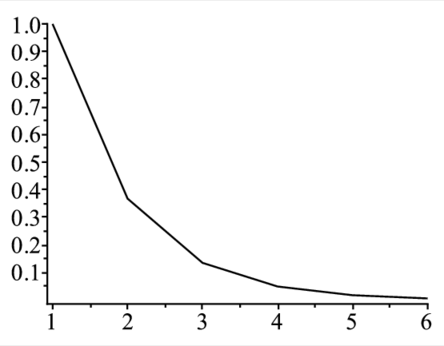

$$ T\, := \,[1,\exp(-1),\exp(-2),\exp(-3),\exp(-4),\exp(-5)] $$

以下のようにoptionをつけるとpointで描く．

> listplot(T,style=point):

それぞれの値の横軸xが1,2,3,..では不都合なときには，2次元のlistlist構造を用意し，[x[i],y[i]]を入れてpointplot関数で表示する ．

> T:=[seq([i/2,exp(-i/2)],i=0..6)]; 
> pointplot(T,symbol=circle,symbolsize=20);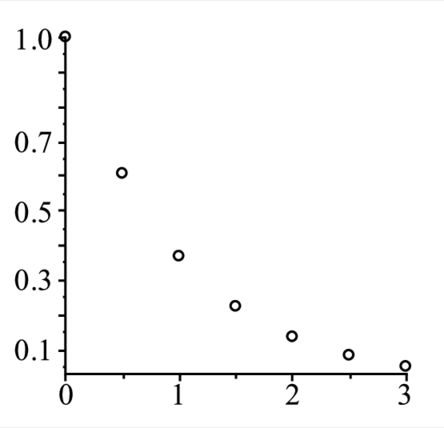

$$ T\, := \,[[0,1],[1/2,\exp(-1/2)],[1,\exp(-1)],[3/2,\exp(-3/2)], \notag \\ [2,\exp(-2)],[5/2,\exp(-5/2)],[3,\exp(-3)]] $$

listplotのように線でつなぎたい時には，以下のようにoptionをつける．

> pointplot(T,connect=true):

写像の表示

ある行列によって点を移動させる写像の様子を示すスクリプトを通して，plottoolsが提供するdisk, arrowの使い方を示す．先ず描画に必要なライブラリーパッケージ(plotsおよびplottools)をwithで読み込んでおく．

> restart; with(plots):with(plottools):

$$ $$

行列$A= \left[ \begin {array}{cc} 1&2\\ 2&1\end {array} \right]$ によって点$a_0$(1, 2)が$a_1$(5, 4)に移動するとする(LinearAlgebra参照）．

> with(LinearAlgebra): A:=Matrix([[1,2],[2,1]]): a0:=Vector([1,2]): a1:=A.a0;

$$ {\it a1}\, := \, \left[ \begin {array}{c} 5\\ 4\end {array} \right] $$

ベクトルが位置座標を意味するようにlistへ変換(convert)する．

> p0:=convert(a0,list):p1:=convert(a1,list):

位置p0に円(disk)を半径0.2,赤色で描く．同じように位置p1に半径0.2，青色でdiskを描く．

> point1:=[disk(p0,0.2,color=red),disk(p1,0.2,color=blue)]:

もう一つ，p0からp1に向かう矢印(arrow)を適当な大きさで描く．後ろの数字をいじると線の幅や矢印の大きさが変わる．

> line1:=arrow(p0,p1,0.05,0.3,0.1):

これらをまとめて表示(display)．このとき，表示範囲を0..6,0..6とする．

> display(point1,line1,view=[0..6,0..6],gridlines=true);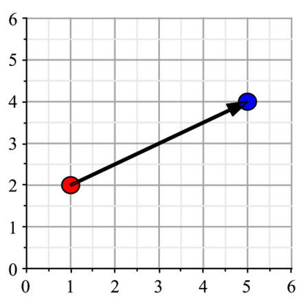

$a_0$(1, 2)の赤点が，$a_1$(5, 4)の青点へ移動していることを示している．

回転写像

次に原点周りでの回転の様子を示す．回転の行列．

> Matrix([[cos(theta),sin(theta)],[-sin(theta),cos(theta)]]);

$$ \left[ \begin {array}{cc} \cos \left( \theta \right) &\sin \left( \theta \right) \\ -\sin \left( \theta \right) &\cos \left( \theta \right) \end {array} \right] $$

これを関数のように定義している．

> A:=t->Matrix([[cos(t),sin(t)],[-sin(t),cos(t)]]);

$$ A\, := \,t\mapsto \left[ \begin {array}{cc} \cos \left( t \right) &\sin \left( t \right) \\ -\sin \left( t \right) &\cos \left( t \right) \end {array} \right] $$

tに回転角(Pi/3)を入れている．

> a0:=Vector([3,0]);
> a1:=A(Pi/3).a0;

$$ {\it a0}\, := \, \left[ \begin {array}{c} 3\\ 0\end {array} \right] \notag \\ {\it a1}\, := \, \left[ \begin {array}{c} 3/2\\ -3/2\,\sqrt {3}\end {array} \right] \notag $$

表示の仕方は，前節と同じ．

> p0:=convert(a0,list):p1:=convert(a1,list):
> point1:=[disk(p0,0.2,color=red),disk(p1,0.2,color=blue)]:
> line1:=arrow(p0,p1,0.05,0.3,0.1):
> display(point1,line1,view=[-4..4,-4..4],gridlines=true);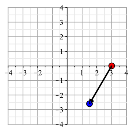

平行投影図の作成

もう少し複雑な対象物として，ここでは立方体の表示を考える．まず３次元座標を打ち込む．

> restart; with(plots): with(plottools): 
  p:=[[0,0,0],[1,0,0],[1,1,0],[0,1,0],
  [0,0,1],[1,0,1],[1,1,1],[0,1,1]]:

$$ $$

次にこれをpointplot3dで簡便に表示．

> points:= { seq(p[i],i=1..8) }:
> pointplot3d(points,symbol=circle,symbolsize=40,color=black);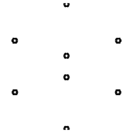

もうすこし見やすいように頂点を結んでおく．たとえば，p[1]とp[2]との間を線で結ぶには，

> line(p[1],p[2]);

とする．それをseqで複数の点間に対して施す．

> ll:=[[1,2],[2,3],[3,4],[4,1],[1,5],[2,6],[3,7],[4,8],
> [5,6],[6,7],[7,8],[8,5]]:
> lines:=[seq(line(p[ll[i][1]],p[ll[i][2]]),i=1..nops(ll))]:
> display(lines,scaling=constrained,color=black);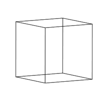

> l3:=display(lines,scaling=constrained,color=black):
> p3:=pointplot3d(p,symbol=circle,symbolsize=40,color=black):
> display([p3,l3],scaling=constrained,color=black);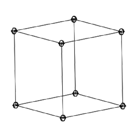

画像をつまんでぐるぐる回してみよ．Mapleではこんな操作は簡単にできるが，よく見ればわかるように，この3次元表示では透視図ではなく，平行投影図といわれるものを書いている．

透視図

透視図のもっとも簡単な変換法は

> proj2d:=proc(x,z) 
    local x1,y1; 
    x1:=x[1]*z/(z-x[3]); 
    y1:=x[2]*z/(z-x[3]);
    return [x1,y1]; 
  end proc:

$$ $$

zに視点の距離を入れて，xで座標を受け取って変換した結果を[x1,y1]として返している．この関数を前の表示と組み合わせれば透視図の描画ができる．

> z_p:=-8:
  lines:=[seq(line(proj2d(p[ll[i][1]],z_p), proj2d(p[ll[i][2]],z_p)), i=1..nops(ll))]:
  display(lines);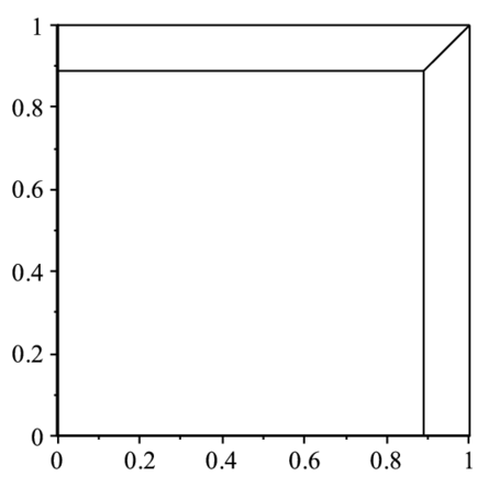

Mapleの描画関数の覚書

mapleにはいくつかの描画レベルに合わせた関数が用意されている．どのような目的にどの関数（パッケージ）を使うかの選択指針として，それぞれがどのような意図で作ら れ，それらの依存関係は以下の通り．

描画の下位関数

plot[structure]にあるPLOT,PLOT3Dデータ構造が一番下でCURVES,POINTS,POLYGONS,TEXTデータを元に絵を描く．

plottoolsパッケージ

PLOTよりもう少し上位で，グラフィックスの基本形状を生成してくれる関数群．arc, arrow, circle, curve, line, point,sphereなどの関数があり，PLOT構造を吐く．表示にはplots[display]を使う．

plotsパッケージ

簡単にグラフを書くための道具．たとえばlistplotは，listデータを簡易に表示する事を目的としている．

animate関数

plotsパッケージにあるanimate関数を使う．構文は以下の通りで，[]内に動画にしたい関数を定義し，tで時間を変えていく．

> with(plots): animate(plot, [sin(x-t),x=0..5*Pi], t=0..10);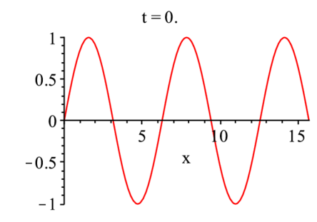

リストに貯めて，display表示

おなじ動作を，display関数でオプションとしてinsequence=trueとしても可能．この場合は第一引数に入れるリスト([])に一連の画像を用意し，コマ 送りで表示させる．

> tmp:=[]: n:=10: for i from 0 to n do t:=i; tmp:=[op(tmp),
> plot(sin(x-t)+sin(x+t),x=0..5*Pi)]; end do:
> display(tmp,insequence=true);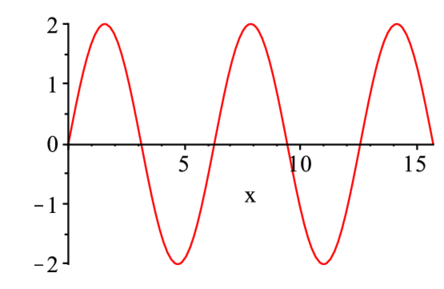

凝った例

ヘルプにある凝った例．Fという動画のコマを吐く関数を用意する．これを，animate関数から適当な変数を入れて呼び出す．backgroundには動かない絵を指定 することができる．

> with(plottools,line): F := proc(t) plots[display](
> line([-2,0],[cos(t)-2,sin(t)],color=blue),
> line([cos(t)-2,sin(t)],[t,sin(t)],color=blue),
> plot(sin(x),x=0..t,view=[-3..7,-5..5]) ); end:
> animate(F,[theta],theta=0..2*Pi, background=plot([cos(t)-2,sin(t),t=0..2*Pi]),
> scaling=constrained,axes=none);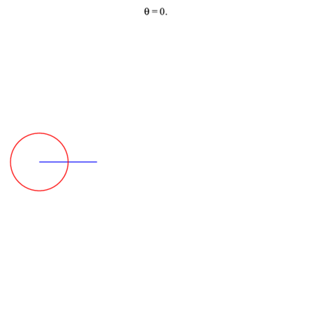

$$ $$

ファイルへの保存

animationなどのgif形式のplotを外部ファイルへ出力して表示させるには，以下の一連のコマンドのようにする．

> plotsetup(gif,plotoutput=file2): display(tmp,insequence=true);
> plotsetup(default):

こいつをquicktimeなどに食わせれば，Maple以外のソフトで動画表示が可能となる．3次元図形の標準規格であるvrmlも同じようにして作成することが可能(?vrml;参照)．